Nov 17, 2018 tags: | computer vision | clustering | visualisation |
Popularity of car colours in the Greater Toronto Area
Updated on Nov 30, 2018
Table of contents
- Summary
- Data collection
- Car detection
- Extraction of car colour information
- Clustering of car colours
- Final result
Summary
According to a survey conducted in 2012 by PPG Industries, white (21%) and black (19%) were the two most popular colours in North America followed closely by silver and grey (16% each). Red and blue accounted for 10 and 8% respectively. I decided to test this data by taking photographs of an intersection in Mississauga, Ontario and analyzing them with the help of YOLOv3 as well as OpenCV and scikit-learn libraries. The results of my analysis (approximately 600 cars) can be summarized by the following bar chart:

Data collection
A Canon PowerShot S100 12 MP camera with CHDK firmware was mounted on a tripod and zoomed on a portion of an intersection from above. Aperture, exposure and white balance were set manually. Photographs were taken automatically every 20 seconds while the battery lasted (approximately 90 min). Photographing was carried out between 2 and 4 pm DST for two days. Unfortunately, seasonal weather changes made it impossible to continue shooting. I manually eliminated the photographs with duplicate objects and was left with 141 unique jpg images at the end.
Car detection
The photographs were batch-cropped (mogrify -crop 4000x2050+0+750 *.jpg) and processed using YOLOv3 (with COCO weights). Originally, I ran YOLOv3 model natively on darknet which required some modifications. Then I discovered that YOLOv3 could be run directly from OpenCV and created scripts for that. If you would like to replicate my project, I recommend using the updated scripts as described below. If you have trouble with your version of OpenCV, you can try my original method.
First you need to download the darknet repository. Either download it as a zip file or use git clone. Assuming you keep git repositories in ~/git, you can run the following commands:
cd ~/git
git clone https://github.com/pjreddie/darknet
cd darknet
wget https://pjreddie.com/media/files/yolov3.weights
The last command downloads the weights of the model trained on the COCO dataset. If you can’t run wget, simply follow the link in your browser and move the weights file to the darknet directory.
Open 1-detect-cars-via-opencv.ipynb and configure the input parameters in each cell before running the notebook. The first cell creates a file listing image paths. The second cell reads each image and runs object detection. The third cell saves the results of object detection.
Extraction of car colour information
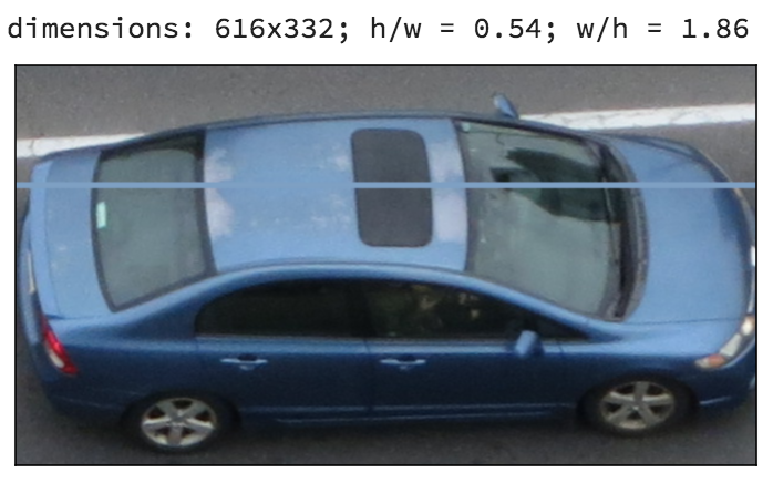
Open 2-extract-colours.ipynb (or 2__outdated__-extract-colours.ipynb if you didn’t use OpenCV for object detection), and configure the path of detected_objects.txt which was saved in the previous notebook. The first cell extracts car objects from the original images, verifies the height:width ratio is within 0.3 and 1 to reject the defective objects, and samples a line of pixels at 30% of the height from the top of the object. K-means is applied to the line array to find 5 colour clusters, and the cluster with the most points is presumed to be the colour of the car, which is appended to an array. The array is saved in the second cell of the notebook.
If you would like to do a dry run on a small batch of randomly selected images set debug = True. This will make the script display each detected object, show its dimensions and the result of colour determination (note: ipython might crash if you try displaying too many objects). Once you are ready to process all objects in a single batch, disable the debug mode.
The image below illustrates successful colour determination.
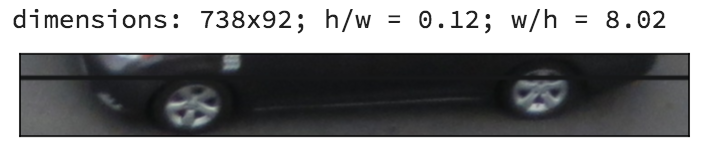
Oddly shaped objects are skipped because K-means clustering often won’t identify the correct colour:
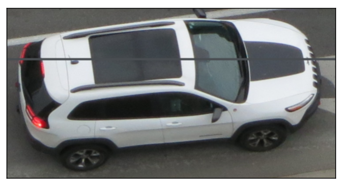
In some cases K-means fails (sort of) even with good images:
The overall colour detection error rate for my dataset was approximately 6%. One limitation of determining colours with K-means clustering is the lack of context. Glare and changing lighting conditions affect the way a colour is encoded by the camera. However, colour perception in humans corrects for such variations by considering the environment. Perhaps I could minimize data variance by identifying the RGB values of some points on the asphalt and then correcting the detected car colours using the same transformation that brings the colour of the asphalt to some standard value. It’s something worth trying in the future (when I get the chance to collect more images).
Clustering of car colours
3-analyze-colours.ipynb contains a collection of scripts implementing a variety of scikit-learn clustering methods. Note: you can replicate the data presented using the supplied detected_colours.npy. I attempted clustering on the standardized data in three different colour spaces (RGB, HCV and L*a*b*). Below is the raw dataset plotted in each of the three coordinate systems.
3D representation in RGB

3D representation in HCV and L*a*b*


It may be easier to explore the data with the following interactive plots generated with three.js (webGL support is required):
Interactive plot in RGB colour space
Interactive plot in HCV colour space
Interactive plot in Lab colour space
The lack of green shades in the dataset makes it possible to project the data points onto a surface with little information loss. The result of SVD in RGB space is presented below:

The parameters of the clustering methods were chosen semi-arbitrarily. The goal was to preserve the distinction between the white, grey and black cars, maintain over 10 shades of grey and have the cluster centers appear in positions that could be mapped to a line in a harmonious arrangement based on hue and brightness. The following plots show the clusters determined as well as their frequencies.
K-means and mean shift in RGB


K-means and mean shift in HCV


K-means and mean shift in L*a*b*


K-means (n=30) in RGB produced a nice arrangement of cluster centres. Unfortunately, the algorithm yielded inaccurate cluster frequencies when checked against black and white cars. K-means in other colour spaces suffered the same fate. The performance of mean shift was even more disappointing.
Agglomerative clustering in RGB
I was able to obtain the most accurate segmentation with agglomerative clustering (Ward’s method).


Agglomerative clustering in HCV


Agglomerative clustering in L*a*b*


Final result
The result of clustering in RGB was easiest to parametrize in one dimension. It was done by first converting the cluster centres from RGB to HSV and getting the index of sorting by V (brightness). Then the index was separated into grey, blue, yellow and red segments (based on hue and saturation) which were then recombined into the final sort index which was used to construct the bar chart.
centers_hsv = rgb2hsv(centers)

# sort by V in HSV
v_sort_ind = np.argsort(centers_hsv[:, 2])

# grey
grey_ind = v_sort_ind[centers_hsv[v_sort_ind,1]<0.25]
# blue
blue_ind = v_sort_ind[(centers_hsv[v_sort_ind,1]>0.25) & (centers_hsv[v_sort_ind,0]>180)& (centers_hsv[v_sort_ind,0]<300)]
# yellow
yel_ind = v_sort_ind[(centers_hsv[v_sort_ind,1]>0.25) & (centers_hsv[v_sort_ind,0]>27) &(centers_hsv[v_sort_ind,0]<150)]
# red
red_ind = v_sort_ind[(centers_hsv[v_sort_ind,1]>0.25) &((centers_hsv[v_sort_ind,0]<27) | (centers_hsv[v_sort_ind,0]>300))]

sort_ind = np.concatenate((blue_ind[::-1], grey_ind, yel_ind, red_ind[::-1]))
Please note black cars appear grey in the figure above because of reflections and poor visual context. It may be helpful to use the grey frame (the average tone of the asphalt) as the reference.
Suggested post:
How random can you be?